Here’s a brief overview of our Keyword Mashup tool, which in essence takes keywords from up to six data sources and consolidates them into a single, de-duplicated list.
If any of those data sources also provide search volume data, it will include that information too, calculating various statistics about those search volumes for each unique keyword.
How To Use The Keyword Mashup
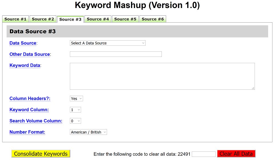
This is what the tool looks like when you first select it from the menu:
 |
As you can see from the top of the screenshot, there are six tabs, representing each of the six data sources that are supported.
For each data source, you need to:
- Select the Data Source from the drop-down list. At the moment, you’ll find the Google Keyword Planner, MerchantWords, and SECockpit, and a few others, but I’ll be adding to this list as time goes on.
- If the Data Source you want is not on that list, then select a value of Other from the drop-down list and then enter the actual name of the Data Source in the Other Data Source box.
- In the Keyword Data box, you need to paste in data that has come from a spreadsheet such as Microsoft Excel. We’ll cover more about how to do this later on, when we walk through an example.
- You need to indicate whether the data you pasted in contains the column headings in the first row. As most do, this is the default option.
- The tool needs to know which column contains the keywords, so select this from the drop-down list. The default is column 1, which is where this information would usually be.
- If the spreadsheet data you pasted in also contains monthly search volume information, then you should tell the tool which column contains that. If there is no search volume information, then you should leave this set to the default value of zero.
- If search volume information is present and it contains either thousands separators or decimal places, then the tool needs to know what format this number uses. The default is American / British, which uses commas for thousands separators and periods / full stops for the decimal point. However, if your spreadsheet uses European format (i.e. periods / full stops for thousands separators, and commas for decimal points), then you can change this setting.
Once you’ve entered this data for each of the Data Sources you have keyword details from, you can click the yellow Consolidate Keywords button.
Alternatively, if you want to clear all the data, then you can enter the Confirmation Code displayed in the box and click the red Clear All Data button. (Filling out all of this information may take a while, which is why we prevent you from clicking the wrong button by mistake.)
Once you’ve submitted your data, the program will process it, and within about 15 seconds, your consolidated keyword details will be displayed, ready for you to copy and paste back into Excel.
The output will show you how many keywords, in total, were processed (from which data sources), and how many unique keywords were found.
Below that, you’ll find a text box that contains all of the consolidated keyword output.
Note that this output is not intended to be read on screen – it needs to be saved or copied and then pasted back into a spreadsheet.
So, you can click in the box to select all data and then manually copy the data to your computer’s clipboard, or you can save a file that contains all the same info.
This file is a tab-separated plain text file, but because it has a file suffix of “.xls”, you should be able to open it directly in Microsoft Excel. You may receive a warning message saying that the file is a different format to the one specified by the file extension, but the file is safe to open.
For each unique keyword, you will see the following information:
- Sources Found, which shows you how many of the data sources you provided data from contained that keyword.
- Minimum Searches, which shows you the lowest number of searches provided by any of the data sources you used.
- Maximum Searches, which shows you the highest number of searches provided by any of the data sources you used.
- Mean Average Searches, which shows you the mean average number of searches provided by all of the data sources you used. The mean average, sometimes called the mathematical average but more commonly known just as the average, is calculated by adding up all of the individual numbers and then dividing by the number of numbers. For example, the mean average of the numbers 1, 2, 3, 4, 5, and 6 is calculated as the sum of those numbers (i.e. 21) divided by how many numbers there are (i.e. 6), giving you an average of 3.5.
- Median Average Searches, which shows you the median average number of searches provided by all of the data sources you used. The Median Average is calculated by listing all of the relevant numbers in ascending numerical order, and then finding the one that is in the middle. For example, the median average of the numbers 5, 2, 7, 9, and 1 is 5 because when you list those five numbers in order, you get 1, 2, 5, 7, and 9, and 5 is the number in the middle. Note that when there is an even number of numbers, e.g. 6, 2, 12, 8, 9, and 3, then the median average is calculated by taking the two middle numbers, which are 6 and 8 in this example (after listing them in ascending numerical order), and then deriving the mean average of those two numbers, which would be 7 in this case.
- Pairs of columns, with one pair for each different Data Source you used, that show whether the keyword was found on that Data Source, and if so, what the search volume was. (Zero will be shown if the keyword was not found on that source, or the keyword was found but no search volume information was present.)
All of this may seem a bit disconnected and obtuse, so…
Let’s Walk Through An Example
If you’d like to follow along with us, you can download this test spreadsheet, which contains keyword data relating to the term “silicone spatula”:
KM-SiliconeSpatulaKeywords.xls
Once you’ve download this and opened it in Excel, we’re ready to begin.
The first tab within the spreadsheet contains the results from data from the Google Keyword Planner.
Make sure the cursor is in the first cell (i.e. A1), and then do a CTRL + A, which will select all of the contents (i.e. in this case, from cell A1 down to cell L1911). You should then use your Copy function (e.g. CTRL + C or click the Copy icon in your toolbar) to copy the data to your clipboard. (Other spreadsheet software will have similar functions.)
Go to the new Keyword Mashup tool, and make sure you’re on the first tab, i.e. Data Source #1.
Select Google Keyword Planner from the drop-down list of Data Sources, and then paste the keyword data from the spreadsheet in the Keyword Data box.
Here are the other settings you should use with this Google Keyword Planner data:
Column Headers?: Yes
Keyword Column: 2
Search Volume Column: 4
Number Format: American / British
Next, go back to the spreadsheet, move to the second tab, which contains data from MerchantWords, and copy the entire contents of that tab too, using the same technique as before.
On the Keyword Mashup tool, click the second tab, i.e. Data Source #2.
Select MerchantWords from the drop-down list of Data Sources, and then paste the keyword data from the spreadsheet in the Keyword Data box.
Here are the other settings you should use with this MerchantWords data:
Column Headers?: Yes
Keyword Column: 1
Search Volume Column: 2
Number Format: American / British
Finally, go back to the spreadsheet one last time, move to the third tab, which contains data from Keyword Snatcher, and copy the entire contents of that tab too, using the same technique as before.
On the Keyword Mashup tool, click the third tab, i.e. Data Source #3.
Select Other from the drop-down list of Data Sources, because Keyword Snatcher isn’t on the list (yet), type in “Keyword Snatcher” in the Other Data Source box, and then paste the keyword data from the spreadsheet in the Keyword Data box.
Here are the other settings you should use with this Keyword Snatcher data:
Column Headers?: No
Keyword Column: 1
Search Volume Column: 0
Number Format: American / British
You should probably double-check that all of the settings are correct on each tab, and then, when you’re ready, click the yellow Consolidate Keywords button.
After a short of delay of approximately six seconds, the screen will be re-displayed with your output.
The first thing you’ll notice is a message telling you how many keywords it processed:
“2,090 keywords were processed from a total of 3 Data Sources (i.e. MerchantWords, and Keyword Snatcher, Google Keyword Planner), which were consolidated down to 1,910 unique keywords.”
The figure at the start of this message shows how many keywords the tool found from the three Keyword Data boxes. (Column headers are not included in this value.)
Next, the Data Sources you specified will be repeated, just for confirmation purposes.
And finally, the figure near the end of the message shows how many unique keywords it found, after consolidating any duplicates.
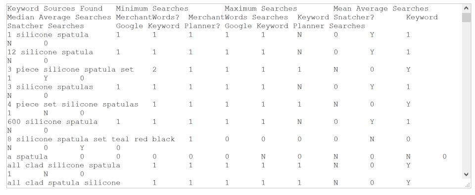
Below that, and the instructions on what to do with this output, you’ll see a box containing all of the consolidated keyword data:
 |
As we said earlier, this box is not mean to be readable on screen – if you’ve used all six Data Sources, then there are a lot of columns of data! Even if you only used a single Data Source, it would still be hard to read.
So, that’s why we’ve given you a few options to copy that data back to Excel, or save the output to your computer.
In the case of this example, if you return to the test spreadsheet and go to the fourth and final tab, which is called Keyword Mashup Output, you’ll see the output from the data you just tested the tool with.
The above instructions (with a link to this blog post) are also shown on the bottom of the Keyword Mashup tool page.
If you have any questions about this tool, then please let me know.


